Algorithm Complexity (Big-O) Explained with Python

In the previous articles, two questions were left hanging. Why is binary search so much faster than linear search? Why does merge sort handle large lists and bubble sort does not? In each case, there was a count of comparisons and a sentence of the type "the work grows with the square of n". This article gives a name and a method to that idea: algorithm complexity, written with Big-O notation.

The question it answers is simple: when the input grows, how much does the work grow? A program that takes an instant with 10 readings may take an eternity with 10 thousand, or may stay instantaneous. Knowing which of the two cases applies before running is one of the most useful skills for anyone who programs, and on the ESP32 it weighs more than on the computer, because the board has far less memory and speed. All the examples below ran in the simulator, and the numbers quoted are the ones it produces. What the computer's Python shows differently is said in the text.

Counting steps instead of seconds

The first idea that comes to mind is to use a stopwatch: run the program and measure how long it took. The problem is that time depends on everything around it. The same function takes one time on the computer, another on the board, another if the computer is busy, and yet another if the simulator is running in a crowded tab. A number in seconds says nothing about the algorithm, only about that run.

The way out is to count steps. You choose the operation that best represents the work, such as a comparison or a turn of a loop, and count how many times it happens as a function of the input size n. The count is the same on any machine. See four functions with very different costs, each returning how many steps it took:

def constante(lista):
    return lista[0], 1

def linear(lista):
    passos = 0
    total = 0
    for v in lista:
        total += v
        passos += 1
    return total, passos

def quadratico(lista):
    passos = 0
    for i in range(len(lista)):
        for j in range(len(lista)):
            passos += 1
    return passos

def logaritmico(n):
    passos = 0
    while n > 1:
        n = n // 2
        passos += 1
    return passos

for n in [10, 20, 40, 80]:
    lista = list(range(n))
    print(n, "O(1):", constante(lista)[1], "O(n):", linear(lista)[1], "O(n^2):", quadratico(lista), "O(log n):", logaritmico(n))
print(logaritmico(1000), logaritmico(1000000), logaritmico(1))
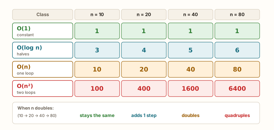
print("end")

The output has four lines, one per size, and then 9 19 0 and end. For n = 10, the first line shows O(1): 1, O(n): 10, O(n^2): 100 and O(log n): 3. For n = 80, they are 1, 80, 6400 and 6. Compare the columns as n doubles from 10 to 20, to 40 and to 80. The O(1) one stays still at 1. The O(log n) one goes up from 3 to 4, 5 and 6, just one step at each doubling. The O(n) one doubles along with it, and the O(n^2) one quadruples: 100, 400, 1600, 6400. (The function names mean constante = constant, quadratico = quadratic and logaritmico = logarithmic.)

That is what Big-O describes. It does not matter whether a step takes a microsecond or a millisecond. What matters is the shape of the curve that the work draws as n grows.

Measuring time also has its place

Counting steps does not replace the stopwatch, it just answers another question. When the doubt is "does this stretch fit in the time I have between two sensor readings?", the answer comes from measuring on the board itself. MicroPython offers time.ticks_ms() and time.ticks_us() for this, and time.ticks_diff() to subtract two instants safely, since the counter wraps around after some time:

import time
print(hasattr(time, "ticks_ms"), hasattr(time, "ticks_us"), hasattr(time, "ticks_diff"))
t0 = time.ticks_ms()
t1 = time.ticks_ms()
d = time.ticks_diff(t1, t0)
print(type(d), d >= 0)
print("end")

The output is True True True, then <class 'int'> True and end. These functions belong to MicroPython. In the computer's Python they do not exist, and there you use time.perf_counter(). The measured values do not appear in the examples of this article because they change on every run, and an output that changes is no use for checking what was learned. The practical rule is to use the count to choose the algorithm and the stopwatch to decide whether it works on the board.

What Big-O describes

Writing O(n) is read "order of n", and says that the work grows proportionally to n. Two rules turn an exact count into a class:

1. Only the term that grows the most counts. If an algorithm makes 3n² + 5n + 2 steps, it is O(n²), because for large n the other terms vanish next to the first.
2. Multiplicative constants do not count. 3n² and n² are in the same class, because tripling the time does not change the shape of the curve.

The table below shows why the first rule works. It calculates 3n² + 5n + 2 and the share that belongs to the 3n² term:

for n in [10, 100, 1000, 10000]:
    total = 3 * n * n + 5 * n + 2
    so_n2 = 3 * n * n
    print(n, total, so_n2, round(100 * so_n2 / total, 2))
print("end")

The output is 10 352 300 85.23, 100 30502 30000 98.35, 1000 3005002 3000000 99.83, 10000 300050002 300000000 99.98 and end. With 10 elements, the 3n² term accounts for 85% of the total. With 10 thousand, for almost 100%. The terms 5n and 2 become a detail, and that is why Big-O throws them away.

This also shows the limit of the notation. O(n²) does not say that an algorithm is slow, it says that it becomes slow when n grows. With few elements, a simple O(n²) can beat a complicated O(n log n). The notation speaks of the algorithm's future, not its present.

The most common classes

Almost everything you write falls into one of these classes, from the cheapest to the most expensive:

O(1), constant. The work does not depend on n. Reading lista[0], reading lista[i], getting len(lista), adding two numbers, looking up a key in a dictionary. In general, also lista.append(x).

O(log n), logarithmic. The work grows slightly, one step each time the size doubles. It is the case of whoever cuts the problem in half at each step, like binary search.

O(n), linear. A loop that goes through each element once. Adding up the list, finding the largest, linear search, x in lista, sum(lista), max(lista).

O(n log n). The typical cost of good sorting algorithms, like merge sort. A little above linear.

O(n²), quadratic. One loop inside another, both going through the list. Bubble, selection and insertion sort, comparing all the pairs.

O(2ⁿ) and similar, exponential. The work doubles, or more, with each extra element. It only serves for tiny inputs. The recursive Fibonacci, further on, is an example.

One way to recognize the class by looking at the code is to count nested loops: with no loop over the input the cost is usually O(1) or O(log n), one loop over n is O(n), two nested are O(n²). But beware of three cautions that counting loops does not catch.

def dois_lacos_seguidos(n):
    passos = 0
    for i in range(n):
        passos += 1
    for j in range(n):
        passos += 1
    return passos

def laco_triangular(n):
    passos = 0
    for i in range(n):
        for j in range(i):
            passos += 1
    return passos

def meio_com_barra(n):
    passos = 0
    while n > 1:
        n = n / 2
        passos += 1
    return passos

def meio_com_duas_barras(n):
    passos = 0
    while n > 1:
        n = n // 2
        passos += 1
    return passos

for n in [10, 20, 40]:
    print(n, dois_lacos_seguidos(n), laco_triangular(n))
print(meio_com_barra(1000), meio_com_duas_barras(1000))
print("end")

The output starts with 10 20 45, 20 40 190 and 40 80 780, and then 10 9 and end. The two consecutive loops make 2n steps, which is still O(n): the two vanishes by the second rule. The nested loops of the triangle, in which the inner one only goes up to i, make n(n-1)/2 steps. It is half the square, and even so it is O(n²): from 20 to 40 elements, the work goes from 190 to 780, about four times. And the last line shows a silent trap: with /, the n becomes a decimal and the loop only ends when the value falls below 1, which gives 10 steps. With //, the integer division stops at 1 and gives 9. The class is the same, but the exact count changes, and the program does not warn. (The names mean dois_lacos_seguidos = two consecutive loops, laco_triangular = triangular loop, meio_com_barra = half with one slash and meio_com_duas_barras = half with two slashes.)

O(log n): cutting the problem in half

The logaritmico from the first example deserves a closer look, because the class is the one least seen in everyday life. It asks: how many times can I divide n in half until I reach 1? For 1000, the answer was 9. For a million, 19. For 1, none, 0.

Notice the size of the jump: from a thousand to a million, a thousand times more elements, the work went from 9 to 19 steps. That is the power of binary search. Searching among a million ordered elements takes about 20 comparisons. Linear search, in the worst case, would take a million. It is the reason sorting, with its cost of O(n log n), pays off when you are going to search the list many times: you pay once, and each search afterwards costs almost nothing.

The logarithm appears whenever a step discards a fraction of what is left, and not a fixed amount. The base of the logarithm, 2, 10 or another, does not matter for Big-O, because changing base only multiplies by a constant. In the examples, division by 2 is used because it is what the algorithms do.

When recursion explodes: Fibonacci

Recursion can hide an enormous cost under short, pretty code. The classic example is Fibonacci, in which each number is the sum of the two before it. The recursive version copies the definition almost word for word, and the loop version keeps only the last two values. Both give the same result, and the program counts the work of each one:

chamadas = 0
def fib(n):
    global chamadas
    chamadas += 1
    if n < 2:
        return n
    return fib(n - 1) + fib(n - 2)

def fib_laco(n):
    a = 0
    b = 1
    passos = 0
    for i in range(n):
        a, b = b, a + b
        passos += 1
    return a, passos

for n in [5, 10, 15, 20]:
    chamadas = 0
    r = fib(n)
    print(n, r, "calls:", chamadas, "| loop:", fib_laco(n))
print("end")

The output has four lines and the end. For n = 5, 5 5 calls: 15 | loop: (5, 5). For n = 10, 10 55 calls: 177 | loop: (55, 10). For 15, 15 610 calls: 1973 | loop: (610, 15). For 20, 20 6765 calls: 21891 | loop: (6765, 20).

The result is the same in both versions, but the work is not. The loop takes n steps. The recursion makes 15, 177, 1973 and 21891 calls, and the ratio between one line and the next stays around 11: each 5 extra units in n multiply the work by about eleven. This is exponential growth. The cause is that fib(n) calls fib(n - 1) and fib(n - 2), and the two recalculate, each on its own, almost everything the other has already calculated. For fib(30), there would be more than 2.6 million calls, and for fib(40), more than 331 million. These two totals come from the formula calculation, not from a run, because the simulator is no place to run that much work.

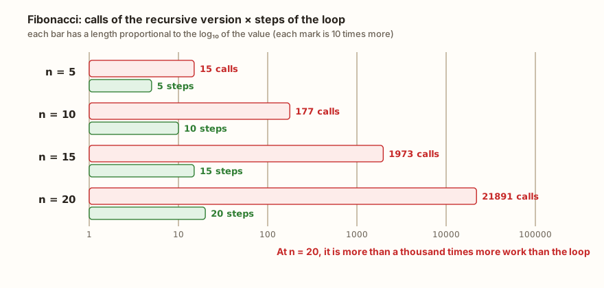
The lesson is not "avoid recursion". Merge sort is recursive and is O(n log n). The lesson is that the shape of the code does not tell the cost: you need to count how many times each piece runs. In Fibonacci, the waste comes from recalculating the same values, and the cure is to store what has already been calculated, either in a loop, or in a dictionary used as memory.

The same problem with three costs

See how the choice of algorithm changes the class of the same problem: finding out whether a list has repeated values. Three ways, each counting its steps:

def duplicados_quadratico(lista):
    comparacoes = 0
    for i in range(len(lista)):
        for j in range(i + 1, len(lista)):
            comparacoes += 1
            if lista[i] == lista[j]:
                return True, comparacoes
    return False, comparacoes

def duplicados_ordenando(lista):
    copia = sorted(lista)
    comparacoes = 0
    for i in range(1, len(copia)):
        comparacoes += 1
        if copia[i] == copia[i - 1]:
            return True, comparacoes
    return False, comparacoes

def duplicados_conjunto(lista):
    vistos = set()
    passos = 0
    for v in lista:
        passos += 1
        if v in vistos:
            return True, passos
        vistos.add(v)
    return False, passos

for n in [10, 100]:
    sem = list(range(n))
    print(n, "no repeats:", duplicados_quadratico(sem), duplicados_ordenando(sem), duplicados_conjunto(sem))
com = [3, 8, 1, 9, 4, 8, 2]
print(duplicados_quadratico(com), duplicados_ordenando(com), duplicados_conjunto(com))
print("end")

The output has three lines and the end. The first, for 10 elements with no repeats, is 10 no repeats: (False, 45) (False, 9) (False, 10). The second, for 100, is 100 no repeats: (False, 4950) (False, 99) (False, 100). The third, with a repeat, is (True, 10) (True, 5) (True, 6). (The names mean duplicados = duplicates, ordenando = sorting, conjunto = set, vistos = seen and sem / com = without / with.)

All three answer correctly, but with different costs. The first compares all the pairs: 45 comparisons with 10 elements and 4950 with 100. It is O(n²), like the triangular loop from the earlier example. The second sorts first, and then the repeats sit side by side, so it is enough to compare each element with the previous one, 9 and 99 comparisons. But these counts do not include the sorting, which costs O(n log n). The total cost of the method is that of the sorting, because it dominates the comparisons. The third uses a set: for each value, it asks whether it has been seen, and the question v in vistos costs O(1) on average. There are 10 and 100 steps, O(n).

The third looks like the winner, and in most cases it is, but it brings a cost that the step count does not show: the set keeps a copy of the values, and that uses memory. On the ESP32, with little memory, trading space for time is not always a good deal. The first method uses almost no memory beyond the list. This is common: there is rarely an algorithm that wins on everything, and choosing is balancing time, memory and simplicity.

Notice also the case of the com list, with the 8 repeated: the methods stopped early, after 10, 5 and 6 steps. That is the best case, when the answer appears before the end. Big-O usually speaks of the worst case, which is that of a list with no repeats, because it is the one that guarantees a limit on waiting. It is what is measured in the table of counts with 10 and 100 elements.

The cost hidden inside a command

Counting loops misleads when a one-line command hides a loop. The most common example is the in applied to a list: x in lista looks like a question, but underneath it is a linear search, O(n). Inside a loop, it becomes O(n²) without the code showing two loops:

def contem(lista, x):
    global comparacoes
    for v in lista:
        comparacoes += 1
        if v == x:
            return True
    return False
comparacoes = 0
def sem_repetidos_lista(dados):
    global comparacoes
    resultado = []
    for x in dados:
        if not contem(resultado, x):
            resultado.append(x)
    return resultado
for n in [10, 100]:
    comparacoes = 0
    r = sem_repetidos_lista(list(range(n)))
    print(n, len(r), comparacoes)
dados = [3, 1, 3, 2, 1]
comparacoes = 0
print(sem_repetidos_lista(dados), comparacoes, sorted(set(dados)))
print("end")

The output is 10 10 45, 100 100 4950, [3, 1, 2] 6 [1, 2, 3] and end. The contem function (contains) plays the role of in and counts the comparisons, so the hidden work is in view. With 10 elements with no repeats, there were 45 comparisons, and with 100, 4950: the same numbers as the quadratic method from the previous section, only now inside a function that, at first sight, has a single loop. The last line shows that the function keeps the order of first appearance ([3, 1, 2]), while sorted(set(dados)) returns the values ordered.

Other commands that hide a loop are sum, max, min, lista.index(x), lista.count(x), lista.remove(x) and the slicing lista[a:b], which copies the elements. All of them cost O(n), and inside a loop over the same list they weigh like a second loop. The in of a set or of a dictionary, on the other hand, costs O(1) on average, and that is why the third method of the previous section stayed linear.

The following example puts it all together in a real ESP32 situation: the moving average of a sensor's last readings. The naive version redoes the sum of the whole window on every reading. The smart one keeps the sum and only updates the ends: it adds the new value and removes the one that left the window.

leituras = [20, 22, 21, 25, 30, 28, 27, 26, 24, 23]
janela = 4

def media_movel_refazendo(dados, k):
    medias = []
    somas = 0
    for i in range(k - 1, len(dados)):
        s = 0
        for j in range(i - k + 1, i + 1):
            s += dados[j]
            somas += 1
        medias.append(s / k)
    return medias, somas

def media_movel_acumulando(dados, k):
    medias = []
    operacoes = 0
    s = 0
    for i in range(len(dados)):
        s += dados[i]
        operacoes += 1
        if i >= k:
            s -= dados[i - k]
            operacoes += 1
        if i >= k - 1:
            medias.append(s / k)
    return medias, operacoes

m1, c1 = media_movel_refazendo(leituras, janela)
m2, c2 = media_movel_acumulando(leituras, janela)
print(m1)
print(m2)
print(m1 == m2, c1, c2)
grandes = list(range(100))
print(media_movel_refazendo(grandes, 10)[1], media_movel_acumulando(grandes, 10)[1])
print(media_movel_refazendo(grandes, 50)[1], media_movel_acumulando(grandes, 50)[1])
print("end")

(The names mean leituras = readings, janela = window, media_movel_refazendo = moving average redoing, media_movel_acumulando = moving average accumulating and grandes = large.) The output starts with the two lists of averages, equal: [22.0, 24.5, 26.0, 27.5, 27.75, 26.25, 25.0]. Then comes True 28 16, the sums done by the two methods on the 10 readings. Then 910 190, for 100 readings and a window of 10, and 2550 150, for a window of 50, and the end.

The two versions give the same answer, and that is the charm: the same problem, the same result, and very different costs. The version that redoes the sum makes (n - k + 1) * k sums, which grows with the window size: 910 with a window of 10 and 2550 with a window of 50. The one that accumulates makes about 2n operations, almost always the same, 190 and 150, because the larger window does not weigh. The first is O(n * k), and the second is O(n). On a board that reads a sensor several times per second, the difference decides whether the program gets the job done.

The algorithms of this part

With the notation at hand, the algorithms of the previous articles are summed up in a table. The columns separate the best and the worst case, because several algorithms behave differently depending on the input:

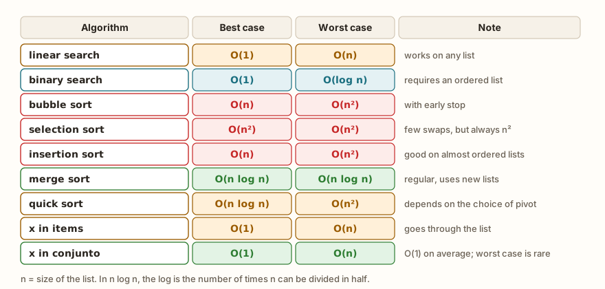
A few points for reading the table carefully:

• Linear search finds it at once if the value is at the start, O(1), and goes through everything if it is at the end or does not exist, O(n).
• Binary search is O(log n), but only works on an ordered list. Sorting costs O(n log n), so it only pays off when you search several times.
• Bubble sort with early stop does O(n) on an already ordered list, a single pass. Selection sort has no such exit: it makes the same comparisons on any list, and what it saves are the swaps.
• Insertion sort is also O(n) when the list is already almost in order. That is why the article about it recommends it for small, almost ordered lists.
• Merge sort keeps O(n log n) on any input, but creates new lists. In the previous article, a reversed list of 1000 elements took 5044 comparisons in merge sort, against 499500 for insertion sort, that second value calculated by the formula.
• Quick sort is O(n log n) on average, but falls to O(n²) in the worst case, when the chosen pivot is always the smallest or the largest element.

The table also recalls an uncomfortable truth: for small lists, everything is fast. The difference between the classes only shows up when n grows. If your list has 20 elements and will never go beyond that, the algorithm that is simplest to understand is often the best.

What Big-O does not say

The notation is a tool, not a verdict, and it is worth knowing its limits:

• It does not measure real time. Two O(n) algorithms can differ by ten times, because Big-O throws away the constants. The stopwatch on the board itself gives the final answer.
• It does not measure memory. The set method won in time and lost in space. There is a space complexity, written with the same notation, and on the ESP32 it matters as much as the time one.
• It does not hold for small n. Constants and smaller terms, which the notation ignores, decide when n is small.
• It depends on the input. That is why there are the best, the average and the worst case, and you need to know which one you are talking about.
• It depends on what is counted. Counting comparisons, swaps or calls gives different numbers, and all are valid as long as you say what the choice was.

On the ESP32: where this weighs

In a sensor program, n is almost never large, but the main loop runs forever. An O(n²) function over 50 readings makes 2500 steps, and if it runs on every cycle, the program spends all its time there. Three situations in which the calculation pays off:

• Average or filter of the last readings. As in the moving average above, redoing the sum on every reading costs O(n * k). Keeping the sum costs O(n).
• Searching a calibration table. If the table is consulted all the time, keeping it ordered and using binary search, or in a dictionary, costs far less than going through it on every query.
• Keeping a history. A list that only grows ends up using up the board's memory. Limiting the size, discarding the oldest, is a decision of space that time Big-O does not see.

In all these cases, the path is the one in the article: count the steps, look at how the count grows, and only then, if the doubt persists, measure on the board with time.ticks_ms().

Common errors

Confusing two loops with O(n²). Two consecutive loops add up, O(n + n), and are still O(n). Only nested ones multiply. Before writing O(n²), check that one loop is really inside the other and that both go through the input size.

Forgetting the hidden loop. x in lista, max, sum and slicing are loops. Counting only the for and while that appear in the code gives a smaller class than the true one.

Failing to count the sorting. When a method starts with sorted(lista), its cost is at least that of the sorting, and not that of the loop that comes afterwards. On the computer, sorted() is O(n log n).

Confusing the best case with the common case. An algorithm that stopped early on the test list may need the whole list on another. Always test the worst case, such as the list with no repeats or the value that does not exist.

Measuring only with small n. With 10 elements, O(n²) and O(n) look the same. Compare counts with n, 2n and 4n, as in the examples, and see what happens when it doubles.

Counting without saying what. A count of "steps" that mixes comparisons and assignments has no meaning. Choose one operation and count only it.

What tends to show up in class

These are patterns that repeat with people learning this subject. They are not the account of a specific class.

Thinking Big-O is a measure of seconds. The person asks "how many seconds is O(n)?". The notation does not answer that, it only says how the work grows. Counting steps, before the stopwatch, helps separate the two ideas.

Memorizing the table without knowing how to count. Whoever memorizes "binary search is log n" but cannot count the steps of a small loop gets stuck on the first different function. Counting by hand, for n = 4 and n = 8, and checking in the simulator teaches more than the table.

Thinking fewer lines is faster. A line with x in lista inside a loop looks leaner than two loops, and costs the same. The size of the code says nothing about the cost.

Ignoring the loop inside the command. The question that helps is: what does this command do underneath? If the answer is "goes through the list", it is a loop.

Wanting the lowest class in everything. Rewriting a 20-element program to gain a class only complicates the code. The right question is whether n will grow.

Exercise: counting steps with user input

Write a program that reads a size n, counts the steps of a simple loop and of two nested loops, and shows the two totals. Then, ask for another n and repeat only the two loops, to see the effect of doubling. Use entradas of 6 and 12 in the simulator, which is what the block below does:

n = int(input("How many elements? "))
passos_um = 0
for i in range(n):
    passos_um += 1
passos_dois = 0
for i in range(n):
    for j in range(n):
        passos_dois += 1
print("n =", n)
print("one loop:", passos_um)
print("two loops:", passos_dois)
n = int(input("And now? "))
passos_dois = 0
for i in range(n):
    for j in range(n):
        passos_dois += 1
print("n =", n, "two loops:", passos_dois)
print("end")

The simulator shows each question followed by the typed value, so the output starts with How many elements? 6. Then come n = 6, one loop: 6, two loops: 36, And now? 12, n = 12 two loops: 144 and end. Notice: n doubled from 6 to 12, and the steps of the double loop went from 36 to 144, four times more, as the table at the start predicted.

To practice, try: swapping the double loop for a triangular one and checking the formula n(n-1)/2; adding a third nested loop and seeing the class become O(n³); counting the steps of a while that divides n by 2; and writing a function that counts the comparisons of linear search in the worst case.

Frequently asked questions

What does the O in Big-O mean? It is the letter for "order": the order of magnitude of the work's growth. O(n²) is read "O of n squared".

What is the difference between O(n) and O(n log n)? The second grows a little faster. For a million elements, n log n is about 20 million, against the million of n. For small lists, it is hardly noticed.

Does O(1) mean a single step? It means that the number of steps does not depend on n. It can be one, two or ten, as long as it does not grow along with the input.

Does the base of the logarithm matter? For Big-O, no. Changing base multiplies by a constant, and constants do not count.

Why does Big-O talk about the worst case? Because it gives a guarantee: the algorithm will never take longer than that. The best case is too optimistic for planning the time of a program.

Is there a Big-O for memory? There is, and it is called space complexity. The set method, for example, uses O(n) of extra space to gain time.

Does MicroPython's sorted() have the same cost as the computer's Python? On the computer, sorted() is O(n log n). MicroPython's implementation is another, as already appeared with stability, and this article does not state its exact cost.

Do I need to know Big-O to program the ESP32? For the first projects, no. But it avoids the shock of a program that works fine with 10 readings and hangs with 1000.

Where to go next

The challenges List Search, Largest in the List and Average of the List are good for counting steps: solve each one and say what the class of your solution is. To review the basics, go through the articles on linear and binary search, bubble and selection sort, insertion sort, merge sort and quick sort, recursion and sets, and through the Logic with Python track.

The next article opens a new part of the series, on objects, errors and good practices, with classes and objects: how to join data and functions into a single thing, with attributes, methods and __init__, and how this organizes a program that grows.