Merge Sort and Quick Sort in Python: Divide and Conquer

The algorithms in the previous article, bubble, selection and insertion, share a limit: the work grows with the square of the list size. For 100 elements, that is about 5 thousand comparisons. For a thousand, almost half a million. There is a smarter idea for larger lists, one that holds across all of computing: divide and conquer. Instead of attacking the whole list, you divide the problem into smaller parts, solve each part in the same way, and join the result.

Two classic sorting algorithms follow this idea, and both use recursion. Merge sort divides the list in half without thinking, sorts the two halves and then merges them. Quick sort chooses an element, the pivot, separates the smaller ones on one side and the larger ones on the other, and sorts each side. The first does its work at the time of joining, and the second, at the time of dividing. This article writes both, measures the cost and shows a limit of the simulator, which imitates the board's, that weighs more on these algorithms than on the previous ones. All the examples ran in the simulator, and the results quoted are the ones it produces.

Merge sort: divide in half, join in order

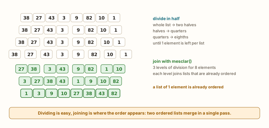
Merge sort rests on a simple operation: taking two lists that are already ordered and joining them into one, also ordered. Since each one is already in order, it is enough to look at the front of both, take the smaller and advance in that list. This is the merge, and the rest of the algorithm is just dividing the list until each piece has one element, which guarantees that the merge always receives ordered lists.

def mesclar(a, b):
    resultado = []
    i = 0
    j = 0
    while i < len(a) and j < len(b):
        if a[i] <= b[j]:
            resultado.append(a[i])
            i += 1
        else:
            resultado.append(b[j])
            j += 1
    resultado.extend(a[i:])
    resultado.extend(b[j:])
    return resultado

print(mesclar([1, 4, 7], [2, 3, 9, 10]))
print(mesclar([], [1, 2]), mesclar([5], []), mesclar([], []), mesclar([2, 2], [2]))

def merge_sort(lista):
    if len(lista) <= 1:
        return lista
    meio = len(lista) // 2
    esquerda = merge_sort(lista[:meio])
    direita = merge_sort(lista[meio:])
    return mesclar(esquerda, direita)

print(merge_sort([38, 27, 43, 3, 9, 82, 10]))
print(merge_sort([3, 3, 1]), merge_sort([]), merge_sort([7]), merge_sort([1, 2, 3]))
original = [5, 2, 4, 1]
print(merge_sort(original), original)

def merge_sort_trace(lista, nivel=0):
    print("  " * nivel + "split", lista)
    if len(lista) <= 1:
        return lista
    meio = len(lista) // 2
    esq = merge_sort_trace(lista[:meio], nivel + 1)
    dir = merge_sort_trace(lista[meio:], nivel + 1)
    r = mesclar(esq, dir)
    print("  " * nivel + "merge", r)
    return r
merge_sort_trace([38, 27, 43, 3])
print("end")

The output starts with [1, 2, 3, 4, 7, 9, 10] and [1, 2] [5] [] [2, 2, 2]. Then come [3, 9, 10, 27, 38, 43, 82], [1, 3, 3] [] [7] [1, 2, 3] and [1, 2, 4, 5] [5, 2, 4, 1]. The trace of the last function is:

split [38, 27, 43, 3]
  split [38, 27]
    split [38]
    split [27]
  merge [27, 38]
  split [43, 3]
    split [43]
    split [3]
  merge [3, 43]
merge [3, 27, 38, 43]

And finally end. (The names mean mesclar = merge, resultado = result, esquerda and direita = left and right, meio = middle and nivel = level.)

The mesclar function uses two indexes, i for the list a and j for b, like two fingers running over two ordered lines. While both fingers are inside the lists, a[i] is compared with b[j], the smaller goes to the resultado, and the finger of that list advances. When one of the lists ends, the rest of the other is left over, which is already in order and only needs to be copied: that is what the two extend lines do, a[i:] and b[j:]. One of the two slices is always empty. The comparison uses <=, and not <, so that, in case of a tie, the element of the left list comes out first, which keeps the sort stable.

The second line of tests shows the edge cases: an empty list, both empty, and repeated values. All of them work.

The merge_sort function is short, and each line has a role:

• if len(lista) <= 1: return lista is the base case of the recursion. A list with zero or one element is already ordered, and there is nothing left to divide.
• meio = len(lista) // 2 finds the cutting point.
• merge_sort(lista[:meio]) and merge_sort(lista[meio:]) sort each half, calling itself with a smaller list. Each call divides again, until it reaches the lists of one element.
• return mesclar(esquerda, direita) joins the two halves, which already come back ordered.

The indented trace shows the order in which things happen. The list [38, 27, 43, 3] is divided into [38, 27] and [43, 3], each into two loose elements. Only when the lists of one element are reached does the work of joining begin: [38] with [27] gives [27, 38], [43] with [3] gives [3, 43], and, finally, the two give [3, 27, 38, 43]. Notice that the print("merge") only appears after the child calls finish, which is recursion in action.

An important detail: merge sort does not change the original list. The slices lista[:meio] and lista[meio:] create new lists, and the result is a new list. That is why original is still [5, 2, 4, 1] after the sorting. It is the opposite of the sort() of lists, which changes in place.

Quick sort: choosing a pivot

Quick sort does the opposite of merge sort: the hard part is dividing, and joining is just concatenating. You choose an element, the pivot, and separate all the others into three groups: those smaller than the pivot, the equal ones and the larger ones. The pivot and its equals are already in the right place. It is enough to sort, in the same way, the group of the smaller and that of the larger, and join everything in the order smaller + equal + larger.

lista = [7, 2, 9, 4, 6, 1, 8]
pivo = lista[len(lista) // 2]
menores = [x for x in lista if x < pivo]
iguais = [x for x in lista if x == pivo]
maiores = [x for x in lista if x > pivo]
print(pivo, menores, iguais, maiores)
def quick_sort(lista):
    if len(lista) <= 1:
        return lista
    pivo = lista[len(lista) // 2]
    menores = [x for x in lista if x < pivo]
    iguais = [x for x in lista if x == pivo]
    maiores = [x for x in lista if x > pivo]
    return quick_sort(menores) + iguais + quick_sort(maiores)
print(quick_sort(menores), quick_sort(maiores), quick_sort(lista))
print("end")

The output is 4 [2, 1] [4] [7, 9, 6, 8], then [1, 2] [6, 7, 8, 9] [1, 2, 4, 6, 7, 8, 9] and finally end. (The names mean pivo = pivot, menores = smaller, iguais = equal and maiores = larger.) It is exactly what the figure shows: the pivot is the 4, the element in the middle, the smaller ones are [2, 1], the larger ones are [7, 9, 6, 8], and each side sorts itself.

The version with comprehensions is the most readable, and a function of a few lines is enough:

def quick_sort(lista):
    if len(lista) <= 1:
        return lista
    pivo = lista[len(lista) // 2]
    menores = [x for x in lista if x < pivo]
    iguais = [x for x in lista if x == pivo]
    maiores = [x for x in lista if x > pivo]
    return quick_sort(menores) + iguais + quick_sort(maiores)

print(quick_sort([38, 27, 43, 3, 9, 82, 10]))
print(quick_sort([3, 3, 1]), quick_sort([]), quick_sort([7]), quick_sort([1, 2, 3]), quick_sort([5, 5, 5]))
original = [5, 2, 4, 1]
print(quick_sort(original), original)

def quick_trace(lista, nivel=0):
    if len(lista) <= 1:
        print("  " * nivel + "done", lista)
        return lista
    pivo = lista[len(lista) // 2]
    menores = [x for x in lista if x < pivo]
    iguais = [x for x in lista if x == pivo]
    maiores = [x for x in lista if x > pivo]
    print("  " * nivel + "pivot", pivo, "smaller", menores, "equal", iguais, "larger", maiores)
    return quick_trace(menores, nivel + 1) + iguais + quick_trace(maiores, nivel + 1)
quick_trace([38, 27, 43, 3, 9, 82, 10])

def particionar(lista, baixo, alto):
    pivo = lista[alto]
    i = baixo
    for j in range(baixo, alto):
        if lista[j] < pivo:
            lista[i], lista[j] = lista[j], lista[i]
            i += 1
    lista[i], lista[alto] = lista[alto], lista[i]
    return i

def quick_no_lugar(lista, baixo, alto):
    if baixo < alto:
        p = particionar(lista, baixo, alto)
        quick_no_lugar(lista, baixo, p - 1)
        quick_no_lugar(lista, p + 1, alto)

dados = [38, 27, 43, 3, 9, 82, 10]
quick_no_lugar(dados, 0, len(dados) - 1)
print(dados)
print("end")

The output starts with [3, 9, 10, 27, 38, 43, 82], then [1, 3, 3] [] [7] [1, 2, 3] [5, 5, 5] and [1, 2, 4, 5] [5, 2, 4, 1]. The trace of quick_trace is:

pivot 3 smaller [] equal [3] larger [38, 27, 43, 9, 82, 10]
  done []
  pivot 9 smaller [] equal [9] larger [38, 27, 43, 82, 10]
    done []
    pivot 43 smaller [38, 27, 10] equal [43] larger [82]
      pivot 27 smaller [10] equal [27] larger [38]
        done [10]
        done [38]
      done [82]

Then come [3, 9, 10, 27, 38, 43, 82] from the in-place version and end.

The quick_sort function has the same design as merge sort: the base case is the list with at most one element, and the recursive step calls the function for both sides. The difference is that here the list is not cut at the middle of the position, but by the value of the pivot. The use of three lists, with iguais apart, is what makes the function handle repeated values well, like [5, 5, 5], and avoids a silent error that we will see later.

The trace holds a lesson. On the first call, the element in the middle is the 3, which happens to be the smallest value in the list. The list of the smaller ones is empty, and that of the larger ones has almost everything, six elements out of seven. The division was uneven: little gain. On the next call it happens again, with the pivot 9. Only after that does the division become reasonable. When the pivot falls near the middle of the values, the two halves have similar sizes and the algorithm is fast. When it falls near one end, each step removes only one or two elements, and the algorithm becomes, in practice, as slow as the simple ones. The choice of pivot is, therefore, the central decision of quick sort.

The quick_no_lugar (in place) version shows the classic variant, which sorts the list itself without creating new lists. The particionar (partition) function uses the last element as the pivot and rearranges the stretch from baixo (low) to alto (high) so that the smaller ones stay on the left, the pivot in the middle and the larger ones on the right. The variable i marks where the next "smaller" goes. At the end, the pivot is swapped to position i, which is its definitive position, and the function returns that position. The recursion then sorts the two stretches, without including the pivot. It is more economical in memory, but requires care with the indexes.

How much they cost

comparacoes = 0
def mesclar(a, b):
    global comparacoes
    resultado = []
    i = 0
    j = 0
    while i < len(a) and j < len(b):
        comparacoes += 1
        if a[i] <= b[j]:
            resultado.append(a[i])
            i += 1
        else:
            resultado.append(b[j])
            j += 1
    resultado.extend(a[i:])
    resultado.extend(b[j:])
    return resultado
def merge_sort(lista):
    if len(lista) <= 1:
        return lista
    meio = len(lista) // 2
    return mesclar(merge_sort(lista[:meio]), merge_sort(lista[meio:]))
def insertion_comparacoes(lista):
    c = 0
    for i in range(1, len(lista)):
        chave = lista[i]
        j = i - 1
        while j >= 0:
            c += 1
            if lista[j] > chave:
                lista[j + 1] = lista[j]
                j -= 1
            else:
                break
        lista[j + 1] = chave
    return c
for n in [8, 16, 100, 1000]:
    inv = list(range(n, 0, -1))
    ord_ = list(range(1, n + 1))
    comparacoes = 0
    r1 = merge_sort(inv)
    ci = comparacoes
    comparacoes = 0
    r2 = merge_sort(ord_)
    co = comparacoes
    print(n, "merge reversed", ci, "ordered", co, "| insertion reversed", insertion_comparacoes(inv[:]) if n <= 100 else "-")
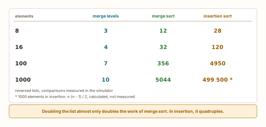
print("end")

The output has four lines: 8 merge reversed 12 ordered 12 | insertion reversed 28, 16 merge reversed 32 ordered 32 | insertion reversed 120, 100 merge reversed 356 ordered 316 | insertion reversed 4950 and 1000 merge reversed 5044 ordered 4932 | insertion reversed -, followed by end. For 1000 elements, insertion was not measured, and the - marks that. The calculation by the formula, n * (n - 1) / 2, gives 499 500 comparisons, about a hundred times more than the 5044 of merge sort.

Merge sort has a very regular behavior. There are about log2(n) levels of division: 3 for 8 elements, 4 for 16, 7 for 100 and 10 for 1000. At each level, the merge goes through all the elements once, which gives something close to n comparisons per level. The total is on the order of n * log2(n): for 100 elements, that product gives about 660, and the 356 measured comparisons are below that. The initial order of the list hardly matters to merge sort: 356 against 316 comparisons for the reversed list and the ordered one.

Comparing with insertion shows the gain. With 8 elements, the difference is small, 12 against 28. With 100, it is 356 against 4950. Each time the list doubles, merge sort does a little more than double the work, and insertion quadruples it. This difference in pace is the subject of the next article, on algorithm complexity.

Quick sort has a similar cost when the pivot divides well, and the same quadratic behavior as the simple algorithms when it divides badly. Since the result depends on the list and on the pivot, we will not tabulate numbers for it here. The next section shows the problem in practice.

The recursion limit and the worst case of quick sort

The article on recursion showed that MicroPython has a much smaller recursion limit than the computer's Python, and that the simulator reproduces this: around 50 nested calls. For merge sort, this is not a problem, because the depth is log2(n): with a thousand elements, 10 levels. For quick sort, it depends on the pivot:

def quick_sort_primeiro(lista):
    if len(lista) <= 1:
        return lista
    pivo = lista[0]
    menores = [x for x in lista[1:] if x < pivo]
    maiores = [x for x in lista[1:] if x >= pivo]
    return quick_sort_primeiro(menores) + [pivo] + quick_sort_primeiro(maiores)
ultimo = 0
for n in range(40, 70):
    try:
        quick_sort_primeiro(list(range(n)))
        ultimo = n
    except RuntimeError:
        print("first error at n =", n, "last ok =", ultimo)
        break
print("end")

The output is first error at n = 51 last ok = 50 and end. (The name quick_sort_primeiro means quick sort with the first element as the pivot, and ultimo means last.)

This version uses the first element as the pivot, and the test is with already ordered lists, from 40 to 69 elements. In an ordered list, the first element is always the smallest: the list of the smaller ones is empty, and that of the larger ones contains all the rest. Each call removes one element, and the depth of the recursion becomes n. In the simulator, the list of 50 elements passes, and the one of 51 blows the limit with RuntimeError, as the output shows. In the computer's Python, the default limit is about a thousand calls, and a list of 100 elements passes with no error.

This shows two things. First, the worst case of quick sort is not theory: it is an ordered list with the pivot at the end, precisely the list that is most common to receive. Second, on the ESP32 the recursion limit brings this worst case much closer than on the computer. With the pivot in the middle, as in the comprehension version, the ordered list is the best case, because the element in the middle divides the list into two equal parts. That is why the earlier quick_sort sorts a reversed list of a thousand elements with no problem, and merge sort too, with 10 levels.

Whoever needs safety chooses a better pivot, such as the middle one, or the median of three (the middle value among the first, the central and the last). But the simplest starting point is this: for small lists and ordinary sorting, use sorted(). The two algorithms in this article are for understanding the idea.

On the ESP32: merging two records ordered by time

Merging two ordered lists is a useful operation on its own, with no need for the whole merge sort. Imagine two sensors that record readings with the instant of each one, each with its list already in time order, and a program that needs a single record, in chronological order:

def mesclar(a, b):
    resultado = []
    i = 0
    j = 0
    while i < len(a) and j < len(b):
        if a[i][0] <= b[j][0]:
            resultado.append(a[i])
            i += 1
        else:
            resultado.append(b[j])
            j += 1
    resultado.extend(a[i:])
    resultado.extend(b[j:])
    return resultado
sensor_a = [(1, "A:21.5"), (4, "A:21.7"), (7, "A:22.0")]
sensor_b = [(2, "B:55%"), (3, "B:56%"), (9, "B:54%")]
for t, msg in mesclar(sensor_a, sensor_b):
    print(t, msg)
log = mesclar(sensor_a, [(4, "B:58%")])
print(log)
print("end")

The output is 1 A:21.5, 2 B:55%, 3 B:56%, 4 A:21.7, 7 A:22.0, 9 B:54%, then [(1, 'A:21.5'), (4, 'A:21.7'), (4, 'B:58%'), (7, 'A:22.0')] and end.

The function is the same, with one change: each item is a tuple (instant, message), and the comparison looks at the first field, a[i][0] against b[j][0]. The result is the record of both sensors interleaved by time. The last test shows the tie-break: when two records have the same instant, 4, the one from list a comes out first, thanks to the <=. The same goes for joining records from files, from two tasks or from two sources of events. The sensors used in the articles on DHT22, HC-SR04 and PIR are examples of sources that can generate these records.

There is a caveat about memory. Merge sort and the quick sort version with comprehensions create new lists on each division, and a board's memory is small. For lists of dozens of items, this weighs nothing. For hundreds or thousands, it is worth thinking about the in-place version, or simply about sorted().

Common errors

The first is forgetting the base case:

def merge_sort(lista):
    meio = len(lista) // 2
    return merge_sort(lista[:meio]) + merge_sort(lista[meio:])
print(merge_sort([3, 1, 2]))

RuntimeError: maximum recursion depth exceeded

Before that line, the simulator prints about 50 repeated lines of File "main.py", line 3, in merge_sort. The function divides and calls itself without ever stopping: a list of one element becomes an empty list, which becomes another empty list, forever. In the computer's Python, the message is RecursionError: maximum recursion depth exceeded while calling a Python object. The fix is the if len(lista) <= 1: return lista.

The second is a merge loop without the stop condition:

def mesclar(a, b):
    resultado = []
    i = j = 0
    while True:
        if a[i] <= b[j]:
            resultado.append(a[i]); i += 1
        else:
            resultado.append(b[j]); j += 1
    return resultado
print(mesclar([1], [2]))

IndexError: list index out of range

With while True, the indexes grow until they pass the end of one of the lists, and the program fails. The correct condition is while i < len(a) and j < len(b), followed by the extend with what is left.

Silent traps

The most dangerous errors of the two algorithms are the ones that give no message:

def quick_sort_ruim(lista):
    if len(lista) <= 1:
        return lista
    pivo = lista[0]
    menores = [x for x in lista if x < pivo]
    maiores = [x for x in lista if x > pivo]
    return quick_sort_ruim(menores) + [pivo] + quick_sort_ruim(maiores)
print(quick_sort_ruim([3, 1, 3, 2, 3]))
def mesclar(a, b):
    r = []
    i = j = 0
    while i < len(a) and j < len(b):
        if a[i] <= b[j]:
            r.append(a[i]); i += 1
        else:
            r.append(b[j]); j += 1
    return r
print(mesclar([1, 4, 7], [2, 3, 9, 10]))
def mesclar_certa(a, b):
    r = []
    i = j = 0
    while i < len(a) and j < len(b):
        if a[i] <= b[j]:
            r.append(a[i]); i += 1
        else:
            r.append(b[j]); j += 1
    return r + a[i:] + b[j:]
print(mesclar_certa([5, 1], [4, 2]))
print("end")

The output is [1, 2, 3], then [1, 2, 3, 4, 7], then [4, 2, 5, 1] and finally end. (ruim means bad and certa means right.)

In the first case, quick_sort_ruim separates only smaller and larger, without keeping the equals. The list [3, 1, 3, 2, 3] has five elements, and the result, three: the two repeated 3s vanished, because neither x < pivo nor x > pivo catches them. The result looks ordered and has the wrong size. That is why the correct version has the iguais list.

In the second, mesclar forgets to copy what was left over after one of the lists ends. The values 9 and 10, which remained in b, vanished: the result has five elements, and the lists added up to seven. The right version ends with r + a[i:] + b[j:].

The third shows a requirement that the function does not check: mesclar assumes that the two lists are already ordered. With [5, 1] and [4, 2], which are not, the result is [4, 2, 5, 1], with no error and no order. Merging does not sort: it joins two things that were already in order.

What tends to show up in class

These are patterns that repeat with people learning these algorithms. They are not the account of a specific class.

Forgetting the base case. The function calls itself until it blows up. The question that helps is: what is the smallest list I know how to sort by doing nothing?

Forgetting to join the result. Writing merge_sort(lista[:meio]) without storing or using what it returns. The function runs, but the ordered list is lost, because merge sort in this form does not change the list in place.

Losing what was left over in the merge. The result comes without the largest elements, and whoever looks only at the start of the list does not notice. Comparing the len of the result with the sum of the sizes is a quick test.

Losing the repeats in quick sort. Separating only smaller and larger, without a list of equals. The error only appears with repeated values, and test lists usually have all different values.

Thinking that quick sort is always fast. Whoever only tests with shuffled lists never sees the worst case. An already ordered list, with the pivot at the first element, is the test that reveals it.

Expecting recursion to work for any size. On the computer, the limit is about a thousand calls. On the board, and in the simulator, the recursion limit is much smaller, and the same code can fail.

Confusing merging with sorting. The merge only works with ordered lists. Calling mesclar with unordered lists returns an unordered list.

Wanting to use these algorithms instead of sorted(). In practice, it is the opposite: you write by hand to understand, and use the ready-made function in the program.

Exercise: sorting with merge sort and finding the median

Write a program that reads the quantity n of numbers, then the n values, sorts them with merge sort and shows the list before and after and the median. The block uses entradas= to provide 6 numbers: 38, 27, 43, 3, 9 and 82.

def mesclar(a, b):
    resultado = []
    i = 0
    j = 0
    while i < len(a) and j < len(b):
        if a[i] <= b[j]:
            resultado.append(a[i])
            i += 1
        else:
            resultado.append(b[j])
            j += 1
    resultado.extend(a[i:])
    resultado.extend(b[j:])
    return resultado
def merge_sort(lista):
    if len(lista) <= 1:
        return lista
    meio = len(lista) // 2
    return mesclar(merge_sort(lista[:meio]), merge_sort(lista[meio:]))
n = int(input())
valores = []
for i in range(n):
    valores.append(int(input()))
ordenados = merge_sort(valores)
print("before", valores)
print("after", ordenados)
print("median", ordenados[n // 2])
print("end")

The simulator repeats the typed values in the output, one per line, and then come before [38, 27, 43, 3, 9, 82], after [3, 9, 27, 38, 43, 82], median 38 and end.

The program keeps the list valores (values) intact, because merge sort returns a new list, and shows both. The median, for an even quantity of numbers like these six, is the average of the two in the middle, 27 and 38. The line ordenados[n // 2] takes only the element at position 3, the 38, which serves for odd quantities and is an approximation for even ones. To practice, try: calculating the right median for even quantities, with the average of the two central values; swapping merge sort for sorted() and comparing; sorting from largest to smallest, swapping the <= for >= in the merge; and counting how many comparisons the merge makes.

Frequently asked questions

Is merge sort better than quick sort? It depends. Merge sort has a regular cost and is stable, but uses new lists. In-place quick sort uses little memory, but can degenerate with a bad pivot.

Why is merge sort stable? Because, on a tie, the merge takes the element of the left list first, with <=. This way the equal ones keep the order in which they came in.

Which pivot should I choose in quick sort? The element in the middle is a good simple choice, and works well with already ordered lists. More robust is the median of three. The first or last element is the worst choice for lists that usually come ordered.

Does sorted() use one of these algorithms? Python uses an algorithm of its own, a hybrid, that combines ideas from merging and insertion. MicroPython's is another, and is not stable, as the article on lambda, map, filter and sorted showed.

Why recursion, if there are loops? Because the idea of dividing and solving smaller parts is naturally recursive. It is possible to write both without recursion, with a stack of your own, but the code becomes much longer.

Do these algorithms suit small lists? They do, but they do not pay off. For a few elements, insertion sort or sorted() are simpler and equally fast.

Where to go next

The challenges Sum of the List, Largest in the List and Reversed List practice the walk and the building of new lists that the merge uses. To review the basics, it is worth going through the articles on recursion, functions with def, bubble and selection sort and insertion sort, and through the Logic with Python track.

The next article closes this part with algorithm complexity, Big-O notation: how to give a name to what was seen here, the work that grows with the square of n in the simple algorithms and with n * log2(n) in merge sort.